For some years now I have been playing around with a certain problem in portfolio statistics: suppose you observe \(n\) independent observations of a \(p\) vector of returns, then form the Markowitz portfolio based on those returns. What then is the distribution of what I call the 'signal to noise ratio' of that Markowitz portfolio, defined as the true expected return divided by the true volatility. That is, if \(\nu\) is the Markowitz portfolio, built on a sample, its 'SNR' is \(\nu^{\top}\mu / \sqrt{\nu^{\top}\Sigma \nu}\), where \(\mu\) is the population mean vector, and \(\Sigma\) is the population covariance matrix.
This is an odd problem, somewhat unlike classical statistical inference because the unknown quantity, the SNR, depends on population parameters, but also the sample. It is random and unknown. What you learn in your basic statistics class is inference on fixed unknowns. (Actually, I never really took a basic statistics class, but I think that's right.)
Paulsen and Sohl made some progress on this problem in their 2016 paper on what they call the Sharpe Ratio Information Criterion. They find a sample statistic which is unbiased for the portfolio SNR when returns are (multivariate) Gaussian. In my mad scribblings on the backs of envelopes and scrap paper, I have been trying to find the distribution of the SNR. I have been looking for this love, as they say, in all the wrong places, usually hoping for some clever transformation that will lead to a slick proof. (I was taught from a young age to look for slick proofs.)
Having failed that mission, I pivoted to looking for confidence intervals for the SNR (and maybe even prediction intervals on the out-of-sample Sharpe ratio of the in-sample Markowitz portfolio). I realized that some of the work I had done on the Asymptotic distribution of the Markowitz Portfolio could be adapted to this purpose. In fact I had even done much of the work when I made the last revision to that paper, back in 2015. This would not be a slick excursion, however, rather hand to hand combat with lots of matrices and the covariances of matrices; kronecker products of Greek letters; a whole hairball of symmetrizing matrices that only Jan Magnus would love. And I got a result, and I pushed it out as version 4 of the paper.
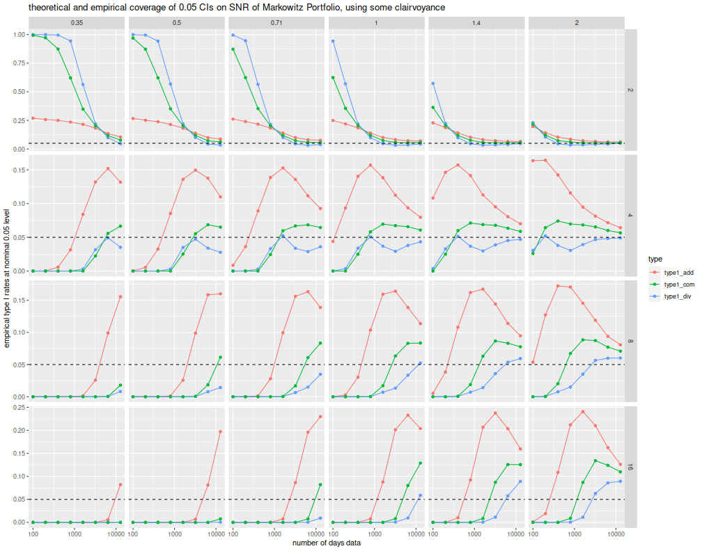
And yet it sucks, to paraphrase Galileo. The confidence intervals are plainly terrible. Below I perform a number of simulations, for 100 to 12800 days (50 year!) of daily data, for 2 to 16 stocks, and for true optimal squared SNR ranging from 0.125 to 4 per year. At each setting I perform 25K simulations, drawing from Gaussian population. (As an efficiency hack, for each setting of the number of stocks and days, the whole spectrum of optimal SNR are tested simultaneously, and so will not have independent errors.)
I then compute the lower 0.05 asymptotic confidence interval as quouted in the paper, based on the difference between the SNR and the observed in-sample optimal Sharpe (which is related to Hotelling's \(T^2\) statistic). I compute another confidence interval based on the ratio of those two statistics. These confidence intervals are computed most optimistically, using the unknown population maximal SNR, as if one were clairvoyant, rather than some sample estimate. I compute a third confidence interval which is the average of the additive and geometric.
suppressMessages({
  library(dplyr)
  library(tidyr)
  library(tibble)
  # https://cran.r-project.org/web/packages/doFuture/vignettes/doFuture.html
  library(doFuture)
  registerDoFuture()
  plan(multiprocess)
})

# one simulation of n periods of data on p assets with true optimal
# SNR of (the vector of) pzeta
onesim <- function(pzeta,n,p) {
  pmus <- pzeta / sqrt(p)
  # simulate an X: too slow.
  #X <- matrix(rnorm(n*p,mean=pmus[1],sd=1),ncol=p)
  #smu1 <- colMeans(X)
  #ssig <- ((n-1)/n) * cov(X)
  # this is faster:
  smu1 <- rnorm(p,mean=pmus[1],sd=1 / sqrt(n))
  ssig <- rWishart(1,df=n-1,Sigma=diag(1,ncol=p,nrow=p)) / n  # sic n
  dim(ssig) <- c(p,p)

  smus <- outer(smu1,pmus - pmus[1],FUN='+')
  smps <- solve(ssig,smus)
  szeta <- sqrt(colSums(smus * smps))
  psnr <- pmus * as.numeric(colSums(smps) / sqrt(colSums(smps^2)))
  cbind(pzeta,szeta,psnr)
}
# do that many times.
repsim <- function(nrep,zetas,n,p) {
  foo <- replicate(nrep,onesim(pzeta=zetas,n,p))
  baz <- aperm(foo,c(1,3,2))
  dim(baz) <- c(nrep * length(zetas),dim(foo)[2])
  colnames(baz) <- colnames(foo)
  invisible(as.data.frame(baz))
}
manysim <- function(nrep,zetas,n,p,nnodes=7) {
  if (nrep > 4*nnodes) {
    # do in parallel.
    nper <- table(1 + ((0:(nrep-1) %% nnodes)))
    retv <- foreach(i=1:nnodes,.export = c('zetas','n','p','repsim','onesim')) %dopar% {
      repsim(nrep=nper[i],zetas=zetas,n=n,p=p)
    } %>%
      bind_rows()
  } else {
        retv <- repsim(nrep=nrep,zetas=zetas,n=n,p=p)
  }
  retv
}

# actually do it many times.
ope <- 252
zetasq <- c(1/8,1/4,1/2,1,2,4) / ope
zeta <- sqrt(zetasq)

params <- tidyr::crossing(tibble::tribble(~n,100,200,400,800,1600,3200,6400,12800),
                          tibble::tribble(~p,2,4,8,16))

nrep <- 25000

set.seed(2356)
system.time({
results <- params %>%
  group_by(n,p) %>%
    summarize(sims=list(manysim(nrep=nrep,zetas=zeta,n=n,p=p))) %>%
  ungroup() %>%
  tidyr::unnest()
})
##    user  system elapsed
##     862    1213     283
kurty <- 1
# summarize the moments:
sumres <- results %>%
  mutate(diffo=psnr - szeta) %>%
  group_by(pzeta,n,p) %>%
    summarize(emp_mean_szeta=mean(szeta),emp_var_szeta=var(szeta),
              emp_mean_szetasq=mean(szeta^2),emp_var_szetasq=var(szeta^2),
              emp_mean_psnr=mean(psnr),emp_var_psnr=var(psnr),
              emp_mean_diffo=mean(diffo),emp_var_diffo=var(diffo)) %>%
  ungroup() %>%
  mutate(bit1 = (kurty*pzeta^2 + 1) * (1 - p),
         bit2 = (3 * kurty - 1) * (pzeta^2/4) + 1) %>%
  mutate(thr_mean_psnr=pzeta + bit1 / (2 * pzeta * n)) %>%
  mutate(thr_mean_szeta=pzeta - bit2 / (2 * pzeta * n)) %>%
  mutate(thr_mean_diffo=(bit1 + bit2) / (2 * pzeta * n)) %>%
  mutate(thr_mean_weird=-(pi/4) * (thr_mean_psnr - pzeta) / pzeta) %>%
  mutate(thr_var_szeta=bit2 / n) %>%
  mutate(thr_var_szetasq=(4 * pzeta^2 + 2 * pzeta^4) / n) %>%
  mutate(thr_var_diffo=thr_var_szeta) %>%
  tidyr::gather(key=series,value=value,matches('^(thr|emp)_'))  %>%
  tidyr::separate(series,into=c('flavor','stat','metric')) %>%
  mutate(flavor=case_when(.$flavor=='emp' ~ 'empirical',
                          .$flavor=='thr' ~ 'theoretical')) %>%
  mutate(zyr=signif(pzeta * sqrt(ope),digits=2))

# confidence intervals and coverage:
cires <- results %>%
  mutate(bit1 = (kurty*pzeta^2 + 1) * (1 - p),
         bit2 = (3 * kurty - 1) * (pzeta^2/4) + 1) %>%
  mutate(ci_add = szeta + ((bit1 + bit2) / (2 * n * pzeta)) + qnorm(0.05) * sqrt(bit2/n)) %>%
  mutate(ci_div = szeta * (1 + ((bit1 + 3 * bit2) / (2 * n * pzeta * pzeta)) + qnorm(0.05) * sqrt(bit2 / (n*pzeta*pzeta)))) %>%
  mutate(ci_com = 0.5 * (ci_add + ci_div)) %>%
  group_by(pzeta,n,p) %>%
    summarize(type1_add = mean(psnr < ci_add),
              type1_div = mean(psnr < ci_div),
              type1_com = mean(psnr < ci_com)) %>%
  ungroup() %>%
  mutate(zyr=signif(pzeta * sqrt(ope),digits=2))
# plot CIs:
library(ggplot2)
ph <- cires %>%
  tidyr::gather(key=type,value=type1,matches('^type1_')) %>%
  ggplot(aes(n,type1,color=type)) +
  geom_line() + geom_point() +
  facet_grid(p ~ zyr,scales='free') +
  scale_x_log10() +
  geom_hline(yintercept=0.05,linetype=2) +
  labs(x='number of days data',
       y='empirical type I rates at nominal 0.05 level',
       title='theoretical and empirical coverage of 0.05 CIs on SNR of Markowitz Portfolio, using some clairvoyance')
print(ph)

I suppose that conceivably, the confidence intervals will asymptotically achieve the nominal coverage. After all, I make no claims about the rate of convergence in the sample size. And there is no reason to think the rate of convergence is uniform across population parameters. However, nobody has enough data to make these confidence intervals even remotely trustworthy; they're a load of dingo's kidneys.
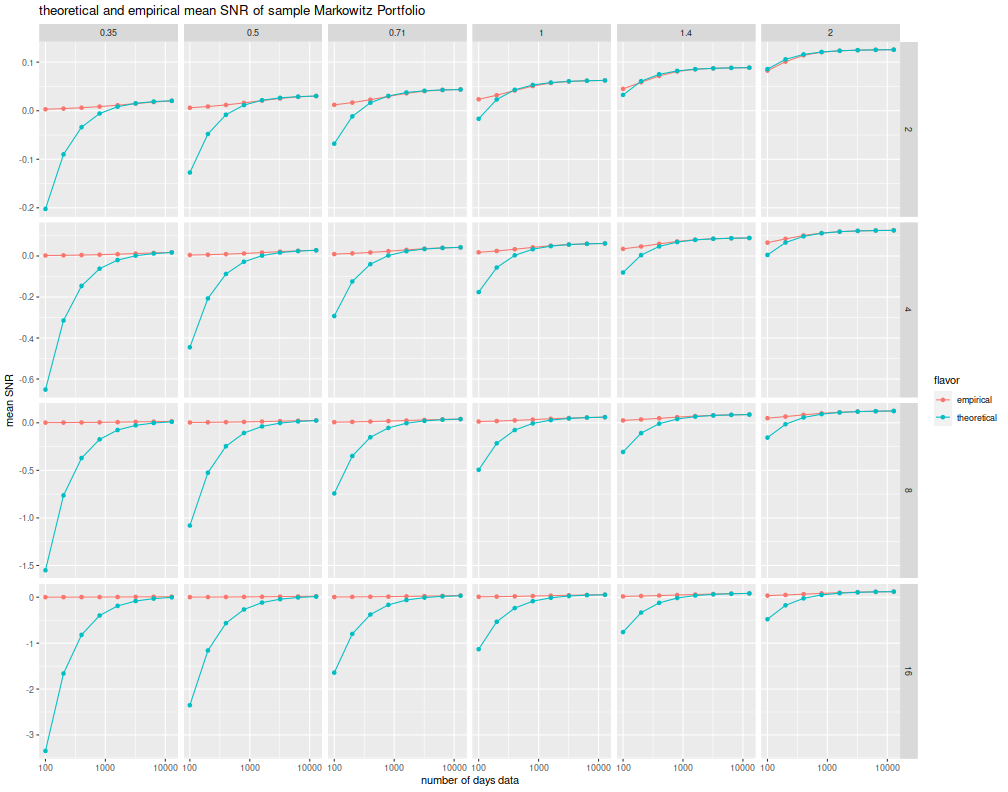
Looking forward, you can plainly see there are a few problems with these results. For one, the asymptotic distribution of Hotelling's \(T^2\) which I am effectively using here, has terrible performance for the small \(n\) case. Well-known distributional results based on the non-central \(F\) should be used instead. However, the distribution of the Markowitz SNR itself is also pretty poor, as shown in the plots below, using the same simulations. Sure, they might make work asymptotically (and I have my doubts), but are useless in our world.
# plot mean snr:
library(ggplot2)
ph <- sumres %>%
  filter(metric=='psnr',stat=='mean') %>%
  ggplot(aes(n,value,color=flavor)) +
  geom_line() + geom_point() +
  facet_grid(p ~ zyr,scale='free') +
  scale_x_log10() +
  labs(y='mean SNR',x='number of days data',
       title='theoretical and empirical mean SNR of sample Markowitz Portfolio')
print(ph)

I was worried that I had solved my problem and wouldn't know what to do with myself anymore. (That's not true, I'm supposed to be working on my book.) The good news, and also the bad news, is that I can continue to work on this problem.