I have been thinking about Elo ratings recently, after analyzing my tactics ratings. I have a lot of questions about Elo: is it really predictive of performance? why don't we calibrate Elo to a quantitative strategy? can we really compare players across different eras? why not use an extended Kalman Filter instead of Elo? etc. One question I had which I consider here is, "what is the standard error of Elo?"

Consider two players. Let the difference in true abilities between them be denoted \(\Delta a\), and let the difference in their Elo ratings be \(\Delta r\). The difference in abilities is such that the odds that the first player wins a match between them is \(10^{\Delta a / 400}\). Note that the raw abilities and ratings will not be used here, only the differences, since they are only defined up to an arbitrary additive offset.

When the two play a game, both their scores are updated according to the outcome. Let \(z\) be the outcome of the match from the point of view of the first player. That is \(z=1\) if the first player wins, \(0\) if they lose, and \(1/2\) in the case of a draw. We update their Elo ratings by

where \(k\) is the \(k\)-factor (typically between 10 and 40), and \(g\) gives the expected value of the outcome based on the difference in ratings, with

Because we add and subtract the same update to both players' ratings, the difference between them gets twice that update, thus the \(2\).

Let \(\epsilon\) be the error in the ratings: \(\Delta r = \Delta a + \epsilon\). Then the error updates as

Using Taylor's Theorem, linearize the function \(g\) to get approximately

Now note that the expected value of \(z\) is exactly \(g\left(\Delta a \right)\). Let \(\sigma^2\) be the variance of \(z\). We have defined an AR(1) process on \(\epsilon\). It's asymptotic expected value is zero, thus the Elo rating difference is unbiased. The asymptotic variance is

Let's test this here. We will assume that \(z\) is \(1/2\) with fixed probability \(p\). (Note that more than half of high level tournament matches end in draws.) This implies that \(z=1\) with probability \(g\left(\Delta a\right) - p\) and equals zero otherwise. The variance of \(z\) is

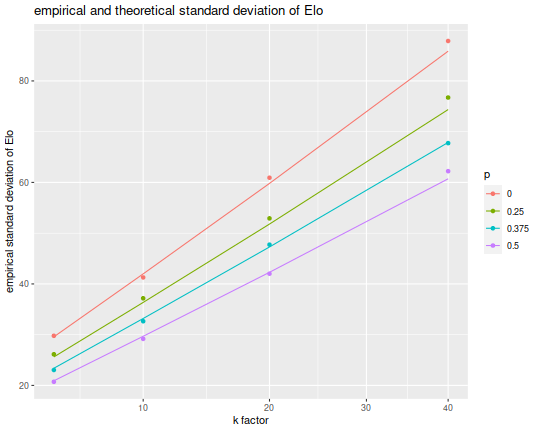
Now I set up a simulation for fixed \(\Delta a\), \(k\), and \(p\) and compare the standard deviation of the rating error to the empirical value. I perform simulations for varying values of \(p\), the probability of a tie, as well as varying \(k\) values. I simulate 50,000 matches for each setting of the parameters, then measure the empirical standard deviation, plotting as a point. The theoretical values are drawn as lines. Note that the theory is based on the linear approximation from Taylor's theorem, so there should be some discrepancy between the two of them.

gfunc <- function(x) { 
  lod <- 10^(x/400) 
  lod / (1 + lod)
}
gprime <- function(x) { (log(10)/400) * gfunc(x) * (1 - gfunc(x)) }

ratsim <- function(nsim=10000,delta_a=0,k=10,p=0.5,delta_r=0) {
  sims <- rep(0,nsim)
  probs <- c(1-gfunc(delta_a)-0.5*p,p,gfunc(delta_a)-0.5*p)
  zvals <- sample(c(0,0.5,1),size=nsim,replace=TRUE,prob=probs)
  for (mmm in 1:nsim) {
    delta_r <- delta_r + 2 * k * (zvals[mmm] - gfunc(delta_r))
    sims[mmm] <- delta_r 
  }
  # recall that epsilon is Delta r - Delta a
  retv <- sims - delta_a
  retv
}

library(tibble)
library(tidyr)
library(dplyr)

set.seed(1234)
simv <- tribble(~k,~p,~delta_a,
                5,0,0,
                10,0.25,0,
                20,0.375,0,
                40,0.5,0) %>%
  complete(k,p,delta_a) %>%
  group_by(k,p,delta_a) %>%
    mutate(empirical=list(sd(ratsim(nsim=50000,delta_a=delta_a,k=k,p=p)))) %>%
  unnest() %>%
  ungroup() %>%
  mutate(sigmasq=gfunc(delta_a) * (1 - gfunc(delta_a)) - (p/4)) %>%
  mutate(theoretical=sqrt(k*sigmasq / (gprime(delta_a) * (1 - k * gprime(delta_a)))))


library(ggplot2)
library(forcats)

ph <- simv %>% 
  mutate(p=forcats::fct_reorder(factor(p),empirical,.desc=TRUE)) %>%
  ggplot(aes(x=k,y=empirical,colour=p)) +
  geom_point() + 
  geom_line(aes(y=theoretical)) + 
  scale_x_sqrt() + 
  labs(x='k factor',y='empirical standard deviation of Elo',
       title='empirical and theoretical standard deviation of Elo')

print(ph)

Note that for very large values of \(p\), which suppresses the variance of \(z\), and for small values of \(k\) we see standard deviation on \(\epsilon\) around 30. Note this is the standard deviation on the error of the differences in ratings. The Elo rating for a player should have smaller error around it, smaller by a factor of \(1/\sqrt{2}\). Thus a standard deviation of around 20 Elo points is to be expected for a player whose \(k\) factor is \(10\), with the error growing like the square root of \(k\).