We have been invited to a champagne tasting party and competition. The rules of the contest are as follows: partygoers bring a bottle of champagne to share. They taste, then rate the different champagnes on offer, with ratings on a scale of 1 through 10. The average rating is computed for each bottle, then divided by the price (plus some offset) to arrive at an adjusted quality score. The champagne with the highest score nets a prize, and considerable bragging rights, for its owner. Presumably the offset is introduced to prevent small denominators from dominating the rating, and is advertised to have a value of around $25. The 'price' is, one infers, for a standard 750 ml bottle.
I decided to do my homework for a change, rather than SWAG it.
I have been doing a lot of web scraping lately, so it was pretty
simple to gather some data on champagnes
from wine dot com. This file includes the advertised and sale prices,
as well as advertised ratings from Wine Spectator (WS), Wine Enthusiast
(WE), and so on. Some of the bottles are odd sizes, so I compute the
cost per liter as well. (By the way, many people would consider the data
collection the hard part of the problem. rvest made it pretty easy, though.)
Here's a taste:
library(dplyr)
library(magrittr)
champ <- read.csv('../data/champagne.csv')
champ %>% arrange(price_per_liter) %>% head(10) %>% kable(format='markdown')
| name | price | sale_price | WS | WE | WandS | WW | TP | JS | ST | liters | price_per_liter |
|---|---|---|---|---|---|---|---|---|---|---|---|
| Pol Clement Rose Sec | 8.99 | NA | NA | NA | NA | NA | NA | NA | NA | 0.75 | 12.0 |
| Freixenet Carta Nevada Brut | 8.99 | NA | NA | NA | NA | NA | NA | NA | NA | 0.75 | 12.0 |
| Wolf Blass Yellow Label Brut | 8.99 | NA | NA | NA | NA | NA | NA | NA | NA | 0.75 | 12.0 |
| Barefoot Bubbly Brut Cuvee | 9.99 | NA | NA | NA | NA | NA | NA | NA | NA | 0.75 | 13.3 |
| Charles de Fere Cuvee Jean-Louis Blanc de Blancs Brut | 9.99 | NA | NA | NA | NA | NA | NA | NA | NA | 0.75 | 13.3 |
| Bellafina Prosecco | 9.99 | NA | NA | NA | NA | NA | NA | NA | NA | 0.75 | 13.3 |
| Jaume Serra Cristalino Extra Dry Cava | 10.00 | 7.99 | NA | NA | NA | NA | NA | NA | NA | 0.75 | 13.3 |
| Segura Viudas Brut Cava | 10.00 | 8.99 | NA | NA | 89 | NA | NA | NA | NA | 0.75 | 13.3 |
| Jaume Serra Cristalino Brut Rose Cava | 10.00 | 8.99 | NA | NA | NA | NA | NA | NA | NA | 0.75 | 13.3 |
| Jaume Serra Cristalino Brut Cava | 10.00 | 8.99 | NA | NA | 88 | NA | NA | NA | NA | 0.75 | 13.3 |
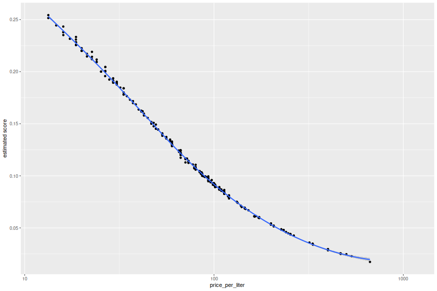
Wine Spectator has the broadest coverage overall, but it seems that W&S has more ratings for the cheaper offerings. Supposing that participant ratings mirrored these snob ratings exactly (up to a multiplicative constant of 10), you arrive at a pretty clear conclusion:
library(ggplot2)
champ$avgrating <- rowMeans(champ[,c('WS','WE','WandS','TP','JS','ST')],na.rm=TRUE)
champ <- champ %>%
    mutate(score=1e-1 * avgrating / (0.75 * price_per_liter + 25))
ph <- ggplot(champ,aes(x=price_per_liter,y=score)) + geom_point() +
    stat_smooth() + scale_x_log10() + labs(y='estimated score')
print(ph)

While I like an analysis that tells me to buy the very cheapest bottle I can find, this is not an airtight strategy. For one, published wine ratings suffer from an insanely compressed range of values. In our sample, the ratings vary from around 87 to 99, depending somewhat on the rating source (and the inter-rater reliability is questionable here). There is also a selection bias involved: presumably the very cheapest champagne would not be rated by any of these tasters, and might score in the 50's or worse if they were. It is hard to imagine that kind of discontinuity, but it is possible. Moreover, in our version, participants are told to rate on a scale of 1 through 10, and presumably may only select an integer. One can easily imagine an outcome of one champagne with an average rating of 8, and another with a rating of 4, only half as good. This is effectively impossible in the professional rating scheme adapted here.
Squashing the range
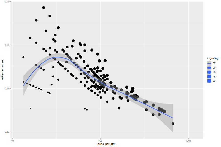
So instead, suppose that suppose that we model our 'schmo' ratings as the 'pro' rating minus 86, capped at 10. Does the analysis change much? Easy to check:
champ <- champ %>%
    mutate(newrating = pmin(10,avgrating - 86)) %>%
    mutate(score=newrating / (0.75 * price_per_liter + 25))
ph <- ggplot(champ,aes(x=price_per_liter,y=score,size=avgrating)) + geom_point() +
    stat_smooth() + scale_x_log10() + labs(y='estimated score')
print(ph)

champ %>% select(name,avgrating,score,price,price_per_liter) %>%
    arrange(desc(score)) %>%
    head(10) %>% kable(format='markdown')
| name | avgrating | score | price | price_per_liter |
|---|---|---|---|---|
| Pere Ventura Cava Tresor Rose | 92.0 | 0.143 | 17 | 22.7 |
| Mionetto Cuvee Sergio Prosecco | 92.0 | 0.133 | 20 | 26.6 |
| Gloria Ferrer Brut | 92.0 | 0.133 | 20 | 26.7 |
| Menage a Trois Prosecco | 91.0 | 0.128 | 14 | 18.7 |
| Ferrari Brut | 92.0 | 0.120 | 25 | 33.3 |
| Segura Viudas Brut Reserva Heredad Cava | 92.0 | 0.120 | 25 | 33.3 |
| Cantine Maschio Prosecco Brut | 91.0 | 0.116 | 18 | 24.0 |
| Roederer Estate Brut | 91.3 | 0.111 | 23 | 30.6 |
| Korbel Brut Rose | 90.0 | 0.108 | 12 | 16.0 |
| Mumm Napa Brut Prestige | 91.0 | 0.106 | 22 | 29.3 |
The sweet spot seems to be at around a 'pro' score of 92, with Pere Ventura winning under this simulation. This is highly dependent on our translation, however. If I had to guess, I would suspect that the Hoi Polloi rating will have mean value somewhat higher than 5, with a definite saturation at 10. Participant's tastes are likely attuned to what they have experienced in the past, so a better SWAG would be to estimate their 'pro' rated history, then map it to a (truncated) normal with mean 6 and standard deviation of 2.5, say. I won't tip my hand, but I am in no way tempted to spend more than 15 bucks on a bottle here.
What else
I should note that the experimental design here is very suspect. The tasting is not even single blind. There seem to be very few controls. Heck, most people will shift their ratings up when they get a little tipsy, so you get a head start if you show up an hour late. I am no expert in market research, but I have conducted this kind of experiment in the past, using a much different protocol and analysis. But that is a story for another time.