I have become more interested in chess in the last year, though I'm still pretty much crap at it. Rather than play games, I am practicing tactics at chesstempo. Basically you are presented with a chess puzzle, which is selected based on your estimated tactical 'Elo' rating, and your rating (and the puzzle's) is adjusted based on whether you solve it correctly. (Without time limit for standard problems, though I believe one can also train in 'blitz' mode.) I decided to look at the data.
I have a few reasons for this exercise:
- To see if I could do it. You cannot easily download your stats from the site unless pay for gold membership. (I skimped and bought a silver.) I wanted to practice my web scraping skills, which I have not exercised in a while.
- To see if the site's rating system made sense as a logistic regression, and were consistent with the 'standard' definition of Elo rating.
- To see if I was getting better.
- To see if there was anything simple I could do to improve, like take longer for problems, or practice certain kinds of problems.
- To look for 'hot hands' phenomenon, which would translate into autocorrelated residuals.
The bad and the ugly
Scraping my statistics into a CSV turned out to be fairly straightforward. The statistics page will look uninteresting if you are not a member. Even if you are, the data themselves are served via JavaScript, not in raw HTML. While this could in theory be solved via, say, phantomJS, I opted to work with the developer console in Chrome directly.
First go to your statistics page in Chrome.
Then conjure the developer console by pressing <CTRL>-<SHIFT>-I.
A frame should appear.
Click on the 'Console' tab, then type in it:
copy(document.body.innerHTML);
This puts the rendered HTML in that page into your clipboard.
Dump it into a CSV (more on this below), then click 'next' on the
page to get the next 50 results, and repeat the process.
I wrote a converter script and a Makefile to simplify this process.
One target of the Makefile dumps the contents of your clipboard
into a randomly named file. Thus once the HTML is in my clipboard,
I can type
make dumpit to dump the data to a file.
I also wrote a converter script to convert the HTML to CSV. The
Makefile knows how to invoke this to convert multiple HTML
files and aggregate them into a single CSV. It also can remove
duplicates, so there's no worries if you go back and repeat
this process, or acidentally dump your clipboard more than once.
This is the Makefile:
ALL_HTML            = $(wildcard chess*.html)
ALL_CSV             = $(patsubst %.html,%.csv,$(ALL_HTML))
BIG_CSV             = tactics_chesstempo.csv

big : $(BIG_CSV) ## convert all html to one big tactics_chesstempo.csv

help:  ## generate this help message
    @grep -P '^(([^\s]+\s+)*([^\s]+))\s*:.*?##\s*.*$$' $(MAKEFILE_LIST) | sort | awk 'BEGIN {FS = ":.*?## "}; {printf "\033[36m%-30s\033[0m %s\n", $$1, $$2}'

$(BIG_CSV) : $(ALL_HTML) converter.r
    r $(firstword $(filter %.r,$^)) -o $@ $(filter %.html,$^)

.PHONY : dumpit

dumpit : ## dump the current clipboard to a html file
    xclip -o > $$(mktemp chess__XXXXXXXXXXXXXXXXXXXXXXXXXXXXXXXX.html)
This is the converter.r script which performs the conversions.
It uses rvest for the heavy lifting of finding and parsing the
HTML table to a dataframe. Some conversions are then performed:
the times are given in an odd format which I convert to seconds,
and so on. Then the data are saved to a file. So after I
have gone through the copy and dump of all my stats, 50 tries at
a time, I then just type
make big, and all the HTML are read, parsed, interpreted,
and written to a CSV file.
# /usr/bin/r
#
# Created: 2017.03.03
# Copyright: Steven E. Pav, 2017
# Author: Steven E. Pav <steven@gilgamath.com>
# Comments: Steven E. Pav

suppressMessages(library(docopt))       # we need docopt (>= 0.3) as on CRAN

doc <- "Usage: converter.r [-v] [-o <OUTFILE>] INFILE...

convert chesstempo ratings html to csv.

-o outfile --outfile=OUTFILE     Where to write the CSV file. [default: -]
-v --verbose                     Be more verbose
-h --help                        show this help text"

opt <- docopt(doc)

library(dplyr)
library(lubridate)
library(readr)

procit <- function(fname) {
  require(dplyr)
  require(rvest)
  require(tidyr)
  # note that if you do not have a Silver membership,
  # your data might not be the 4th table in the page,
  # so you may have to change the [[4]] to a [[3]] or
  # something like that.
  indat <- read_html(fname) %>%
    html_table() %>%
    { .[[4]] } %>%
    setNames(gsub('\\s','_',names(.))) %>%
    rename(N=`#`) %>%
    filter(!grepl('Loading',Time)) %>%
    mutate(N=as.numeric(gsub(',','',N)),
           Time=as.POSIXct(Time),
           ProblemId=as.integer(ProblemId),
           Rating=as.numeric(Rating)) %>%
    tidyr::separate(User_Rating,sep='\\s+',c('end_elo','delta')) %>%
    mutate(end_elo=as.numeric(end_elo),
           delta=as.numeric(gsub('[()]','',delta))) %>%
    mutate(success=delta > 0)
}

hms_to_sec <- function(hmstr) {
  require(lubridate)
  ifelse(grepl('^\\d{1,2}:\\d{2}:\\d{2}$',hmstr),hmstr,paste0('00:',hmstr)) %>%
    lubridate::hms() %>%
    lubridate::period_to_seconds()
}

all_csv <- lapply(opt$INFILE,procit) %>%
  bind_rows() %>%
  distinct(ProblemId,end_elo,delta,.keep_all=TRUE) %>%
  arrange(Time,ProblemId) %>%
  mutate(Av_seconds=hms_to_sec(Av_Time)) %>%
  mutate(Solve_seconds=hms_to_sec(Solve_Time)) %>%
  mutate(After_seconds=hms_to_sec(After_First)) %>%
  mutate(ProblemId=sprintf('%d',as.integer(ProblemId)))

if (opt$outfile=='-') {
  cat(readr::format_csv(all_csv))
} else {
  readr::write_csv(path=opt$outfile,all_csv)
}
How am I doing?
To give some indication of what the data contain, here
is a peek at my most recent attempts. I believe the
timestamps are in UTC. The Rating is the problem's
rating, while end_elo is my rating after attempting
the problem. The delta is the change in rating based
on whether I successfully solved the problem. Then
there are three fields giving, in seconds, the average
time taken by all users for that problem, the time
I took, and the amount of time after my first move it
took to complete the problem. (Sometimes the first move
is obvious, or one does not properly anticipate the
response.)
| Time | ProblemId | Rating | end_elo | delta | success | Av_seconds | Solve_seconds | After_seconds |
|---|---|---|---|---|---|---|---|---|
| 2017-06-27 04:28:28 | 30808 | 1625 | 1939 | 3.4 | TRUE | 95 | 515 | 23 |
| 2017-06-28 02:47:00 | 158098 | 1804 | 1923 | -15.7 | FALSE | 278 | 80281 | 0 |
| 2017-06-29 02:27:34 | 94353 | 1820 | 1931 | 8.2 | TRUE | 241 | 18584 | 11 |
| 2017-07-05 03:15:56 | 152510 | 1831 | 1941 | 9.7 | TRUE | 177 | NA | 64 |
| 2017-07-06 03:11:24 | 155678 | 1966 | 1928 | -12.3 | FALSE | 287 | 86091 | 256 |
| 2017-07-07 03:31:22 | 154471 | 1763 | 1936 | 7.4 | TRUE | 365 | 87371 | 4 |
| 2017-07-08 00:52:11 | 116754 | 1692 | 1941 | 5.2 | TRUE | 544 | 76830 | 19 |
| 2017-07-08 04:00:46 | 73857 | 1825 | 1924 | -16.7 | FALSE | 311 | 11303 | 0 |
| 2017-09-05 06:08:29 | 95229 | 1765 | 1944 | 20.1 | TRUE | 392 | NA | 15 |
| 2017-09-08 03:56:20 | 176378 | 1832 | 1967 | 22.8 | TRUE | 392 | 251187 | 54 |
Regrettably what is missing here is any indication of the 'tags' or 'motifs' of each problem: whether it involves, say, endgame, or a skewer, or a certain kind of mate threat, sacrifice, and so on. I suppose I have to upgrade to gold membership or do some serious scraping to get that information.
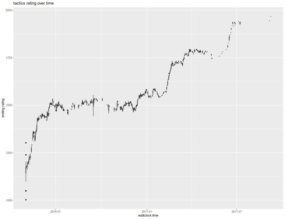
Here is a plot of my progress over time. After a crash course in tactics last summer I got above 1500 and stayed there for a long time. In fact, my goal for 2017 was to surpass 1600 in rating. I figured it might take all year. After a false start, I somehow had some breakthrough in February, and quickly shot through 1600, then 1700. I had been reading 'The Soviet Chess Primer', and started to finally feel like I was learning something. Then I hit another ceiling, stumbling along for three or four weeks trying to best 1725, after which I broke through to the upper 1700s. I am now gunning for 1800, and hope to hit 1850 by year's end.
ph <- indat %>%
    mutate(dayo=lubridate::floor_date(Time,'day')) %>%
    ggplot(aes(dayo,end_elo,group=dayo)) +
    geom_boxplot() +
    labs(y='ending rating',x='wallclock time',title='tactics rating over time')
print(ph)

Lords of logistic
Is the Elo rating really a simple logistic regression? Based on my reading of the wikipedia page, the Elo system aims to assign scores to players such that the log base-10 of the odds that player A beats player B (ignoring the possibility of draws) is \((E_A - E_B) / 400\), where \(E_A, E_B\) are the respective ratings of the two players. Note that this specifies ratings up to an additive constant, which presumably was chosen so that an entry level player has a score of around 1500. The current world champions have an Elo rating of over 2800, while the best chess playing computers are estimated to have ratings over 3000. Translating to tactical problems, and converting to natural log, the natural log odds of solving a problem with rating \(R_p\) given that the player's rating is \(R\) is
The upshot is that a logistic fit of successes against problem rating should
have an coefficient term of approximately -0.006 and an intercept
term of negative that times \(R\). Let us check that with data.
There was a long period of time where my rating was relatively stable, hovering
around 1500. I will use that data to fit a logistic regression. As a friendly
warning, the R function glm does not default to logistic regression, so
I wrote a simple wrapper.
# logistic regression for dummies:
lgreg <- function(formula,data,...) { glm(formula=formula,family=binomial(link="logit"),data=data,...) }

# regression data:
regdat <- indat %>%
  filter(end_elo >= 1475,end_elo <= 1525) %>%
  mutate(deltime=as.numeric(Time - min(Time)) / 86400) %>%
    filter(!is.na(Solve_seconds)) %>%
  mutate(took_long=Solve_seconds > 60)
mod0 <- lgreg(success ~ Rating,data=regdat)

print(summary(mod0))
Call:
glm(formula = formula, family = binomial(link = "logit"), data = data)

Deviance Residuals:
   Min      1Q  Median      3Q     Max
-2.200  -1.191   0.691   0.945   1.514

Coefficients:
             Estimate Std. Error z value Pr(>|z|)
(Intercept)  9.356442   1.085244    8.62  < 2e-16 ***
Rating      -0.006223   0.000765   -8.13  4.2e-16 ***
---
Signif. codes:  0 '***' 0.001 '**' 0.01 '*' 0.05 '.' 0.1 ' ' 1

(Dispersion parameter for binomial family taken to be 1)

    Null deviance: 1164.4  on 895  degrees of freedom
Residual deviance: 1089.8  on 894  degrees of freedom
AIC: 1094

Number of Fisher Scoring iterations: 4
So the slope term with respect to problem ratings is -0.006, close to the nominal value of -0.006. In fact, that nominal value is around 0.61 estimated standard errors from the fit value, nothing unusual. We can also infer my rating over this period from the regression coefficients, computing a value of 1504, about what I would expect given my selection criteria for the data.
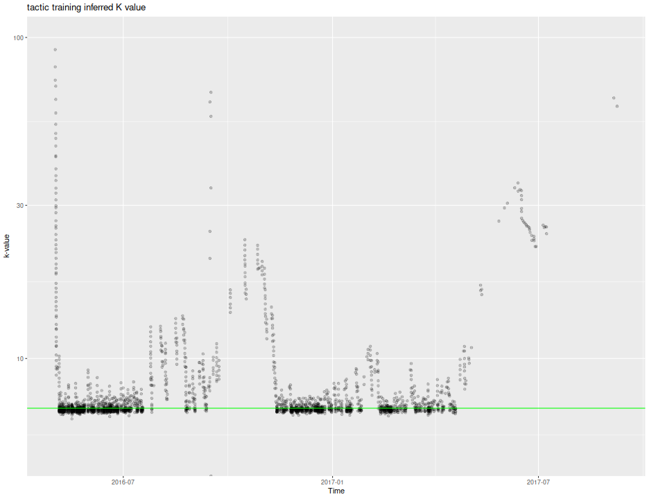
While I am at it, I can compute the so-called 'k-value' that is used to update ratings. Rather than perform a logistic regression using all match data for a user, the Elo rating is computed by adding to one's rating a factor, \(k\) times the 'surprise', which is the outcome as a 0/1 variable minus the expected value of that outcome. A larger value of \(k\) means that the Elo system can 'learn' one's rating faster, but it also means that the Elo rating comes with larger estimation error. The FIDE system uses a \(k\) value between 10 and 40 depending on whether you are a new player, or have reached a certain Elo rating.
I am guessing the same delta which is added (or subtracted if negative) to my Elo is subtracted (added) to the problem rating. (Actually, it is not clear if the problem rating given on the stats page is a snapshot at solve time, or is the current value, or if problem ratings are static. I assume it is a snapshot taken after my attempt at the problem.) I perform that computation, showing the k-value over time, along with a horizontal line at 7, which seems to be the value used by Chesstempo. Note there are some deviations, one during the burn-in period, then another, in September 2016. I remember that period, as it seemed my tactic Elo was highly volatile. Perhaps there was a systematic bug, or the k-value is supposed to change over a user's life-cycle.
ph <- indat %>%
  mutate(pre_rating=Rating+delta,
         pre_elo=end_elo-delta) %>%
  mutate(logodds=(pre_rating-pre_elo)/400) %>%
  mutate(expected=1/(1 + 10^logodds)) %>%
  mutate(surprise=as.numeric(success) - expected) %>%
  mutate(kval=delta/surprise) %>%
  ggplot(aes(Time,kval)) +
  geom_point(alpha=0.2) + scale_y_log10(limits=c(5,100)) +
  geom_hline(yintercept=7,color='green') +
  labs(x='Time',y='k-value',title='tactic training inferred K value')
print(ph)

Is our pawns learning?
Now to consider if I am improving, and to see if I can accelerate my rate of improvement. One piece of advice I read on the forums was to take more time for problems, even an hour or more. I am not sure I can always follow this advice, as there are often diminuishing marginal returns of attention. I might be better off giving up on the problem and learning the solution. There is a tension here between exploration and exploitation, one might say, because my only training is in solving problems: the test is the homework.
Nevertheless, I want to figure out if my recent gains in rating are attributable to: more time spent on problems, in which case there is no diminuishing returns; or on more problems attempted, in which case I should set an upper bound on how long I should look at a problem; or on just time passing, wherein I should get a good night's sleep instead of trying another problem tonight.
To check these, I will use data from Jan 21, 2017 onward. I built a kitchen
sink logistic regression with terms for intercept, problem rating,
number of wallclock days since Jan 21, 2017, number of cumulative hours
spent on problems since that time, and cumulative number of problems
attempted since that time. Note that the Solve_seconds data are a bit
messy, since if I look at a problem, then sleep on it, the value can
be huge. To correct for this, I cap the solve time at 1 hour.
regdat <- indat %>%
  filter(Time >= as.Date('2017-01-21')) %>%
    filter(!is.na(Solve_seconds)) %>%
  mutate(took_long=Solve_seconds > 60) %>%
  arrange(Time) %>%
  mutate(Solve_hours=Solve_seconds/3600) %>%
  mutate(wallclock_days=(1+(as.numeric(Time - min(Time)) / 86400)),
         probs_attempted=(seq_along(Time)),
         cumulative_hours=cumsum(pmin(Solve_hours,1.0)),
         took_long=Solve_seconds/Av_seconds)

mod_clock <- lgreg(success ~ Rating + wallclock_days,data=regdat)
mod_all <- lgreg(success ~ Rating + wallclock_days + cumulative_hours + probs_attempted,data=regdat)
print(summary(mod_all))
Call:
glm(formula = formula, family = binomial(link = "logit"), data = data)

Deviance Residuals:
   Min      1Q  Median      3Q     Max
-2.230  -1.127   0.643   0.852   1.573

Coefficients:
                 Estimate Std. Error z value Pr(>|z|)
(Intercept)       9.44521    1.57859    5.98  2.2e-09 ***
Rating           -0.00624    0.00106   -5.86  4.7e-09 ***
wallclock_days    0.04630    0.01105    4.19  2.8e-05 ***
cumulative_hours -0.06680    0.01669   -4.00  6.3e-05 ***
probs_attempted   0.01818    0.00523    3.48  0.00051 ***
---
Signif. codes:  0 '***' 0.001 '**' 0.01 '*' 0.05 '.' 0.1 ' ' 1

(Dispersion parameter for binomial family taken to be 1)

    Null deviance: 672.37  on 552  degrees of freedom
Residual deviance: 619.33  on 548  degrees of freedom
AIC: 629.3

Number of Fisher Scoring iterations: 4
Looking at that summary, we can convert the effects into effective rating
deltas by dividing by the Rating coefficient. So the coefficient for
wallclock_days translates into an effective Elo delta per day of around
7.421. This
seems insane, but note that if you fit a model to only problem rating and
walllclock, I experienced a more modest Elo delta of around
1.975, which
is not totally crazy. The problem is that the coefficient for cumulative
hours is negative, and I seem to be spending a steady 2 hours a day or
so on chesstempo (my family is considering an intervention). In fact,
the fit coefficients seem to suggest that if I spend more than two hours
a day, my rating will suffer, which I will magically attribute to fatigue.
An ANOVA will confirm that the cumulative_hours is significant in
this regression. However, I suspect that the hockey stick shape in my progress
plot is due to something other than an increase in time spent on problems.
mod_sub <- lgreg(success ~ Rating + wallclock_days + probs_attempted,data=regdat)
print(anova(mod_all,mod_sub,test='Chisq'))
Analysis of Deviance Table

Model 1: success ~ Rating + wallclock_days + cumulative_hours + probs_attempted
Model 2: success ~ Rating + wallclock_days + probs_attempted
  Resid. Df Resid. Dev Df Deviance Pr(>Chi)
1       548        619
2       549        635 -1    -16.2  5.8e-05 ***
---
Signif. codes:  0 '***' 0.001 '**' 0.01 '*' 0.05 '.' 0.1 ' ' 1
A simple regression using the ratio of the time I took for a problem to the average time (with some featurization), does not indicate that I perform better when I take longer, when you take into account the wallclock growth:
mod_took <- lgreg(success ~ Rating + wallclock_days + I(log(pmin(2,took_long))),data=regdat)
print(summary(mod_took))
Call:
glm(formula = formula, family = binomial(link = "logit"), data = data)

Deviance Residuals:
   Min      1Q  Median      3Q     Max
-2.259  -1.247   0.689   0.853   1.521

Coefficients:
                           Estimate Std. Error z value Pr(>|z|)
(Intercept)                 9.54270    1.53617    6.21  5.2e-10 ***
Rating                     -0.00572    0.00100   -5.71  1.1e-08 ***
wallclock_days              0.01170    0.00350    3.34  0.00084 ***
I(log(pmin(2, took_long))) -0.12030    0.21819   -0.55  0.58140
---
Signif. codes:  0 '***' 0.001 '**' 0.01 '*' 0.05 '.' 0.1 ' ' 1

(Dispersion parameter for binomial family taken to be 1)

    Null deviance: 672.37  on 552  degrees of freedom
Residual deviance: 636.08  on 549  degrees of freedom
AIC: 644.1

Number of Fisher Scoring iterations: 4
On Fire
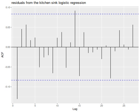
Finally, I can look at some 'hot hands' phenomenon. I take the residuals from
the kitchen sink model, and look at their simple autocorrelation function,
(Note that the forecast package can do this via ggplot2.) I see a negative
first autocorrelation, with some noise. The same general pattern shows for
the wallclock-only regression, not shown. My interpretation is that when I
solve a difficult problem, I get cocky; when I fail on an easy problem, I
become cautious, but the effect wears off immediately.
library(lubridate)
library(ggplot2)
library(forecast)

ph <- ggAcf(residuals(mod_all,type='deviance')) +
    labs(title='residuals from the kitchen sink logistic regression')
print(ph)

In conclusion
No more chess problems tonight: just go to sleep.