In a previous blog post, I looked at two asymptotic confidence intervals for the Signal-Noise ratio of the sample Markowitz portfolio, finding that they generally did not give nominal type I rates even for large sample sizes (50 years of daily data). In a followup post, I looked at the covariance of some elements of the Markowitz portfolio, finding that they seemed to be nearly normal for modest sample sizes. However, in that post, I used the 'TAS' transform to a \(t\) variate, and found, again, that large sample sizes were required to pass the eyeball test in a Q-Q plot.
Here I mash up those two ideas to construct another confidence limit for the Signal Noise ratio. So I take the asymptotic covariance in the Markowitz portfolio elements, and use them with the TAS transform to get a confidence limit. (You can get the gory details around equation (52) of version 5 of my paper, which also contains the simulations below.)
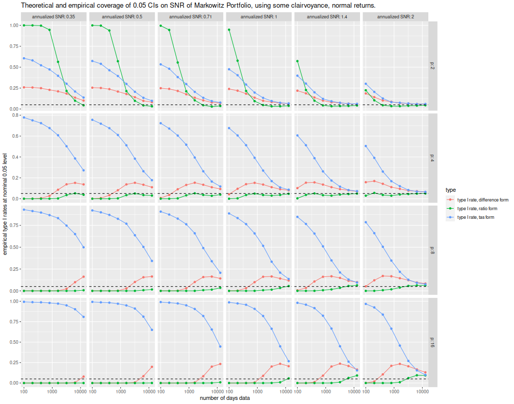
Here we examine all three of those confidence limits, finding that none of them achieve near nominal type I rates. Again, I let \(p\) be the number of assets, \(n\) the number of days observed, \(\zeta\) is the population maximal Signal Noise ratio. Here I am observing multivariate normal returns, so the kurtosis factor is not used here. I perform a number of simulations across different values of these parameters, each time performing 10000 simulations, computing the sample Markowitz portfolio, and its Signal Noise ratio.
suppressMessages({
  library(dplyr)
  library(tidyr)
  library(tibble)
  # https://cran.r-project.org/web/packages/doFuture/vignettes/doFuture.html
  library(doFuture)
  registerDoFuture()
  plan(multiprocess)
})

# one simulation of n periods of data on p assets with true optimal
# SNR of (the vector of) pzeta
onesim <- function(pzeta,n,p) {
  pmus <- pzeta / sqrt(p)
  # simulate an X: too slow.
  #X <- matrix(rnorm(n*p,mean=pmus[1],sd=1),ncol=p)
  #smu1 <- colMeans(X)
  #ssig <- ((n-1)/n) * cov(X)
  # this is faster:
  smu1 <- rnorm(p,mean=pmus[1],sd=1 / sqrt(n))
  ssig <- rWishart(1,df=n-1,Sigma=diag(1,ncol=p,nrow=p)) / n  # sic n
  dim(ssig) <- c(p,p)

  smus <- outer(smu1,pmus - pmus[1],FUN='+')
  smps <- solve(ssig,smus)
  szeta <- sqrt(colSums(smus * smps))
  psnr <- pmus * as.numeric(colSums(smps) / sqrt(colSums(smps^2)))
  cbind(pzeta,szeta,psnr)
}
# do that many times.
repsim <- function(nrep,zetas,n,p) {
  foo <- replicate(nrep,onesim(pzeta=zetas,n,p))
  baz <- aperm(foo,c(1,3,2))
  dim(baz) <- c(nrep * length(zetas),dim(foo)[2])
  colnames(baz) <- colnames(foo)
  invisible(as.data.frame(baz))
}
manysim <- function(nrep,zetas,n,p,nnodes=7) {
  if (nrep > 4*nnodes) {
    # do in parallel.
    nper <- table(1 + ((0:(nrep-1) %% nnodes)))
    retv <- foreach(i=1:nnodes,.export = c('zetas','n','p','repsim','onesim')) %dopar% {
      repsim(nrep=nper[i],zetas=zetas,n=n,p=p)
    } %>%
      bind_rows()
  } else {
    retv <- repsim(nrep=nrep,zetas=zetas,n=n,p=p)
  }
  retv
}

# actually do it many times.
ope <- 252
zetasq <- c(1/8,1/4,1/2,1,2,4) / ope
zeta <- sqrt(zetasq)

params <- tidyr::crossing(tibble::tribble(~n,100,200,400,800,1600,3200,6400,12800),
                          tibble::tribble(~p,2,4,8,16),
                          tibble::tribble(~kurty,1))

nrep <- 10000

set.seed(2356)
system.time({
results <- params %>%
  group_by(n,p,kurty) %>%
    summarize(sims=list(manysim(nrep=nrep,zetas=zeta,n=n,p=p))) %>%
  ungroup() %>%
  tidyr::unnest()
})
   user  system elapsed
352.070 530.625 117.240
Here I collect the simulations together, computing the three confidence limits and then the empirical type I rates. I plot them below.
# the nominal rate:
typeI <- 0.05
# invert the TAS function
anti_tas <- function(x) { x / sqrt(1 + x^2) }

# confidence intervals and coverage:
cires <- results %>%
  mutate(kurty=1) %>%
  mutate(bit1 = (kurty*pzeta^2 + 1) * (1 - p),
         bit2 = (3 * kurty - 1) * (pzeta^2/4) + 1) %>%
    mutate(lam1=pzeta*sqrt((2+3*(kurty-1))/(4*n)),
                 lamp=sqrt(1 + kurty*pzeta^2)/sqrt(n)) %>%
    mutate(tpart=qt(typeI,df=p-1,ncp=szeta/lam1)) %>%
  mutate(ci_add = szeta + ((bit1 + bit2) / (2 * n * pzeta)) + qnorm(typeI) * sqrt(bit2/n)) %>%
  mutate(ci_div = szeta * (1 + ((bit1 + 3 * bit2) / (2 * n * pzeta * pzeta)) + qnorm(typeI) * sqrt(bit2 / (n*pzeta*pzeta)))) %>%
  mutate(ci_tas = pzeta * anti_tas((lam1 * tpart) / (lamp * sqrt(p-1)))) %>%
  group_by(pzeta,n,p,kurty) %>%
    summarize(type1_add = mean(psnr < ci_add),
              type1_div = mean(psnr < ci_div),
              type1_tas = mean(psnr < ci_tas)) %>%
  ungroup() %>%
  mutate(zyr=signif(pzeta * sqrt(ope),digits=2)) %>%
  rename(`annualized SNR`=zyr)
# plot CIs:
library(ggplot2)
ph <- cires %>%
  tidyr::gather(key=type,value=type1,matches('^type1_')) %>%
    mutate(type=case_when(.$type=='type1_add' ~ 'type I rate, difference form',
                                                .$type=='type1_div' ~ 'type I rate, ratio form',
                                                .$type=='type1_tas' ~ 'type I rate, tas form',
                                                TRUE ~ 'bad code')) %>%
  ggplot(aes(n,type1,color=type)) +
  geom_line() + geom_point() +
  facet_grid(p ~ `annualized SNR`,scales='free',labeller=label_both) +
  scale_x_log10() +
  geom_hline(yintercept=0.05,linetype=2) +
  labs(x='number of days data',
       y='empirical type I rates at nominal 0.05 level',
       title='Theoretical and empirical coverage of 0.05 CIs on SNR of Markowitz Portfolio, using some clairvoyance, normal returns.')
print(ph)

The new confidence limit, plotted in blue and called the "tas form" here, is apparently very optimistic and much too high. The empirical rate of type I errors is enormous, sometimes over 90%. It should be noted that the simulations here use some amount of 'clairvoyance' on \(\zeta\); use of a sample estimate would further degrade them, but they are already unusable except for unreasonably large sample sizes. So back to the drawing board.