In a previous blog post I used logistic regression on games played data to estimate the piece value of pieces in Atomic chess. Since then I have been playing less Atomic and more Antichess. In Antichess, you win by losing all your pieces. To facilitate this, capturing is compulsory when possible; when multiple captures are possible you may select among them. There is no castling, and a pawn may promote to a king, but otherwise it is like traditional chess. (For more on antichess, I highly recommend Andrejić's book, The Ultimate Guide to Antichess.)
A king is a relatively powerful piece in Antichess: it can not as easily be turned into a "loose cannon", yet it can move in any direction. In general you want to keep your king on the board and remove your opponent's king. In that spirit, I wanted to estimate piece values in Antichess. I will use logistic regression for the analysis, as I did in my analysis of atomic chess.
For the analysis I pulled rated games data from Lichess. I wrote some code that will download and parse this data, turning it into a CSV file. I am sharing v1 of this file, but please remember that Lichess is the ultimate copyright holder.
The games in the dataset end in one of three conditions: Normal, Time forfeit, and Abandoned (game terminated before it began). The last category is very rare, and I omit these from my processing. The majority of games end in the Normal way, and I will consider only those. Also, games are played at various time controls, and players can make suboptimal moves when pressed for time, so I will restrict to games played with at least two minutes per side.
The game data includes Elo scores (well, Glicko scores, but I will call them Elo) for players, as computed prior to the game. A piece in the hands of a more skilled player will have higher value, and I want to control for this. To avoid cases where the player is new to the system and their Elo has not yet converged to a good estimate, I select only matches where each player has already recorded at least 50 games in the database when the game is played. I also select for Normal terminations, since these are unambiguous victories. The remaining set contains 'only' 5654755 games.
Checking on the data,
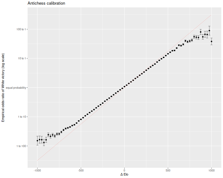
here is a plot of empirical log odds, versus Elo difference, in bins 25 points wide.
This is in natural log odds space, so we expect the line to have slope of
\(\operatorname{log}(10) / 400\) which is around 0.006.
While the empirical data is nearly linear in Elo difference, large differences
in Elo overestimate the certainty of the victory for the stronger player.
That is, the Elo is not well calibrated and exaggerates differences in
ability.

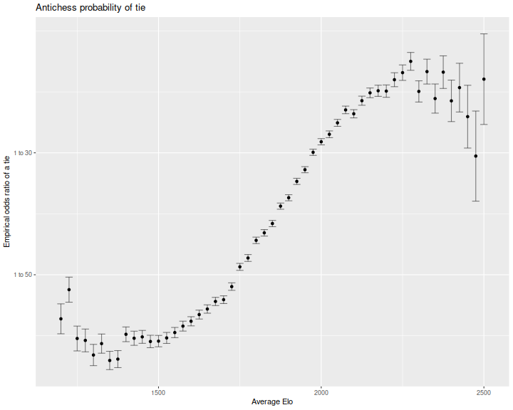
In competitive traditional chess, draws are quite common. I was curious if a similar effect is seen in Antichess. Here is the ratio of odds of a tie, as a function of the average Elo of the two players. The log odds are perhaps increasing in average Elo, but then plateau or decrease at higher levels of play.

Openings
Let us briefly consider openings. It is actually known that Antichess is a winning game for White (!) with opening e2e3. However, the "proof" relies on massive search, and no person could possibly remember all the lines. Do we find that players mostly play this opening? And when they do, does it boost their chances of winning?
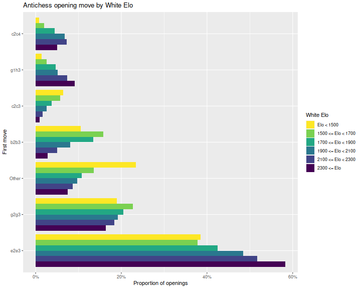
To answer that, here are bar plots of the most frequent opening moves by White, grouped by
White's Elo.
I am not filtering on the outcome in these plots, only Elo, number of games and time controls.
We see that indeed e2e3 is the most commonly played opening, and is played
more by higher Elo players.
The second most popular opening, g2g3 is favored more by lower Elo players.

Recall that Elo is defined so that the log odds of victory from White's perspective is 10 to the Elo difference (White's minus Black's) divided by 400. We expanded this in previous blog posts to include other terms, for example, playing a certain opening move, or having certain pieces still on the board.
Here I perform a logistic regression analysis on our data under the basic model
where \(c\) is in 'units' of Elo. Here is a table of the regression coefficients from that logistic regression, along with standard errors, the Wald statistics and p-values. I also convert the coefficient estimate into Elo equivalent units. White's tempo advantage is equivalent to around 18 extra Elo points. Note that the pre-game Elo is only equivalent to 0.93 Elo points. This is consistent with the plot above, where the pre-game Elo difference exaggerates probability of winning.
| term | estimate | std.error | statistic | p.value | Elo equivalent |
|---|---|---|---|---|---|
| (Intercept) | 0.101 | 0.001 | 84.5 | 0 | 18.00 |
| Elo | 0.005 | 0.000 | 719.5 | 0 | 0.93 |
Logistic analysis of opening moves
Of course, this is only if White does not squander their tempo. Some opening moves are likely to result in a higher boost to White than this average value, and some lower. I will now fit a model of the form
where \(1_{e2e3}\) is a 0/1 variable for whether White played e2e3 as their first move, and \(c_{e2e3}\) is the coefficient which we will fit by logistic regression. By rescaling by the magic number \(\operatorname{log}(10) / 400\), the coefficients \(c\) are denominated in 'Elo units'. Here is a table from that fit:
| term | estimate | std.error | statistic | p.value | Elo equivalent |
|---|---|---|---|---|---|
| Elo | 0.005 | 0.000 | 711.13 | 0 | 0.92 |
| c2c4 | 0.161 | 0.005 | 31.50 | 0 | 28.00 |
| g2g4 | 0.159 | 0.006 | 26.11 | 0 | 28.00 |
| g1h3 | 0.137 | 0.005 | 25.93 | 0 | 24.00 |
| e2e3 | 0.132 | 0.002 | 73.41 | 0 | 23.00 |
| g2g3 | 0.099 | 0.003 | 37.57 | 0 | 17.00 |
| b2b3 | 0.020 | 0.004 | 5.38 | 0 | 3.40 |
| Other | -0.018 | 0.004 | -4.68 | 0 | -3.10 |
Oddly the provably winning move e2e3 does not show as large an effect size as some of the other moves, although it does display greater statistical significance. This is likely because it is played far more often than the other moves, we have more evidence that it gives a non-zero boost to winning chances.
Second moves
The coefficients found here are for average play against these opening moves. Here I perform an analysis of Black's replies to White's opening moves. I filter for White's move, then perform a logistic regression, only considering the most frequent replies. Here is a table of the regression coefficients for three of White's best opening moves. Because the equations are still from White's point of view, Black would choose to play the move with the lowest Elo equivalent. Below we plot the coefficient estimates of Black's replies, again grouping statistically non-distinguishable coefficient estimates.
| move1 | move2 | estimate | std.error | statistic | p.value | Elo equivalent |
|---|---|---|---|---|---|---|
| c2c4 | Elo | 0.005 | 0.000 | 163.221 | 0.000 | 0.90 |
| c2c4 | e7e6 | -0.063 | 0.025 | -2.489 | 0.013 | -11.00 |
| c2c4 | g7g6 | 0.013 | 0.017 | 0.757 | 0.449 | 2.20 |
| c2c4 | c7c6 | 0.066 | 0.014 | 4.739 | 0.000 | 11.00 |
| c2c4 | Other | 0.121 | 0.017 | 7.210 | 0.000 | 21.00 |
| c2c4 | b7b5 | 0.162 | 0.007 | 22.357 | 0.000 | 28.00 |
| c2c4 | d7d5 | 0.446 | 0.014 | 32.091 | 0.000 | 78.00 |
| e2e3 | Elo | 0.005 | 0.000 | 478.357 | 0.000 | 0.93 |
| e2e3 | e7e6 | 0.095 | 0.007 | 13.920 | 0.000 | 16.00 |
| e2e3 | b7b5 | 0.099 | 0.002 | 48.491 | 0.000 | 17.00 |
| e2e3 | c7c5 | 0.252 | 0.007 | 36.701 | 0.000 | 44.00 |
| e2e3 | b7b6 | 0.281 | 0.012 | 22.719 | 0.000 | 49.00 |
| e2e3 | Other | 0.417 | 0.009 | 46.487 | 0.000 | 72.00 |
| e2e3 | a7a6 | 0.442 | 0.015 | 28.780 | 0.000 | 77.00 |
| g2g4 | Elo | 0.005 | 0.000 | 129.990 | 0.000 | 0.87 |
| g2g4 | b7b6 | -0.035 | 0.018 | -1.966 | 0.049 | -6.00 |
| g2g4 | g7g6 | -0.014 | 0.013 | -1.078 | 0.281 | -2.30 |
| g2g4 | c7c5 | 0.056 | 0.035 | 1.591 | 0.112 | 9.60 |
| g2g4 | Other | 0.225 | 0.019 | 12.147 | 0.000 | 39.00 |
| g2g4 | f7f5 | 0.240 | 0.009 | 25.263 | 0.000 | 42.00 |
| g2g4 | h7h5 | 0.437 | 0.020 | 22.023 | 0.000 | 76.00 |
We see that Black's best reply to e2e3 is actually e7e6, but b7b5, the start to the "suicide defense", is also very good.
Piece value
As I did for Atomic chess, I also computed a difference in piece counts at random points over the lifetime of each game. As before, I use logistic regression to estimate the coefficients in the model
where \(\Delta e\) is the difference in Elo, and \(\Delta P, \Delta N, \Delta B, \Delta R, \Delta Q, \Delta K\) are the differences in pawn, knight, bishop, rook, queen and king counts. Here \(p\) is the probability that White wins the match. Because this is Antichess, one expects that having pieces is associated with losing, so I expect to see all the constants \(c\) negative. However, the least negative of them are the more valuable pieces in antichess.
As previously, I subselect to games where each player has already recorded at least 50 games in the database, where both players have pre-game Elo at least 1500, and games which are at least 10 ply in length. As in my analysis of atomic I have computed the differences in piece counts at some pseudo-random snapshot in each game. Thus the values below give a kind of 'average value' of the pieces over an antichess game.
Here is a table of the estimated coefficients for the four regressions, with coefficients and standard errors in Elo equivalents, as well as Wald statistics. The intercept term can be interpreted as White's tempo advantage. We see that, indeed, the King is the least worst piece to have, then a knight, pawn, queen, bishop and rook. Note that the pre-game Elo score still shows an estimated value rather less than 1. There are issues with the Lichess Antichess Elo which should be examined further.
| term | Estimate | Std.Error | Statistic |
|---|---|---|---|
| Elo | 0.856 | 0.001 | 715.4 |
| White Tempo | 16.989 | 0.211 | 80.6 |
| Pawn | -47.034 | 0.138 | -339.7 |
| Knight | -44.921 | 0.264 | -170.2 |
| Bishop | -69.601 | 0.292 | -238.6 |
| Rook | -76.817 | 0.296 | -259.6 |
| Queen | -63.006 | 0.423 | -148.8 |
| King | -9.317 | 0.391 | -23.8 |