Rather than fade into ignominy as a lesser Ralph Nader, Jill Stein has managed to twist the knife in the still-bleeding Left, fleecing a couple of million from some disoriented voters for a recount of the election in Wisconsin, Michigan, and Pennsylvania. While a recount seems like a less likely path to victory for Clinton than, say, a revolt of the Electoral College, or the Donald pulling an Andy Kaufman, perhaps it should be undertaken if there is any evidence of fraud. Recall that prior to the election (and since!) we were warned of the possibility of 'massive voter fraud'. I am not familiar with the legal argument for a recount, but was curious if there is a statistical argument for one. I pursue a simple analysis here.
The arguments that I have heard for a recount (other than the danger to our republic from giving power to mentally unstable blowhard, but I will try to keep my political bias out of here) sounded pretty weak, as they could easily be explained away by an omitted variable. For example, arguments of the form "Trump outperformed Clinton in counties with electronic voting machines," even if couched in a 'proper' statistical test, are likely to be assuming independence of those events, when they need not be independent for numerous reasons.
Instead, I will fall back here to a weaker analysis, based on Benford's Law. Benford's Law, which is more of a stylized fact, states that the leading digit of naturally occurring collections of numbers should follow a certain distribution. Apparently this method was used to detect suspicious patterns in the 2009 Iranian elections, so you would expect only an amateur ballot-stuffer would expose themselves to this kind of diagnostic.
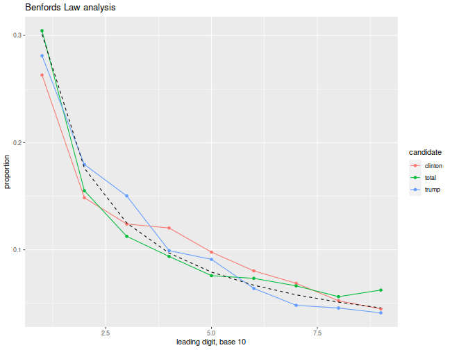
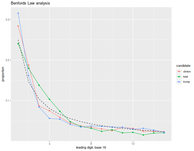
First I grab the ward by ward Wisconsin voter data. This set is marked 'Under Recount', so I am sure it is the best data. I load the excel (!) spreadsheet, and rename some columns. After some mumbo jumbo to define the digit functions and the expected distribution for the same, I make plots of the leading digit, base 10, of the count of Clinton votes, Trump votes, and total votes, across the wards, along with the 'expected' distribution of the same under Benford's Law. Because Benford's Law is applicable under alternative numerical representations (there is nothing special about 10), I also plot the same using a base 16 representation, below.
require(readxl)
require(dplyr)
require(tidyr)
require(ggplot2)

cdata <- readxl::read_excel('Ward_by_Ward_Report_President_0.xlsx',
    sheet='Ward by Ward Report',
    skip=10) %>%
    setNames(gsub('\\s','_',names(.)))
colnames(cdata)[1] <- 'County_possibly'
colnames(cdata)[2] <- 'ward'
colnames(cdata)[3] <- 'total'

cdata <- cdata[!(cdata$total < 1),]

# function which computes the distribution of first digits of x mod m
first_digit <- function(x,m=10) {
    maxb <- floor(log(x,base=m))
    leadd <- floor(x / (m^maxb))
    return(leadd)
}
dbenford <- function(x, m=10) {
    return(log((1+(1/x)),base=m))
}

ben_data <- function(cdata,mybase=10) {
    all_d <- cdata %>%
        select(total,ward,`Donald_J._Trump__Michael_R._Pence`,`Hillary_Clinton__Tim_Kaine`) %>%
        setNames(c('total','ward','trump','clinton')) %>%
        tidyr::gather(key='candidate',value='votes',total,trump,clinton)

    sub_d <- all_d %>%
        dplyr::filter(votes > 0) %>%
        mutate(firstd=first_digit(votes,m=mybase)) %>%
        group_by(candidate,firstd) %>%
            summarize(nfirst=n()) %>%
        ungroup()

    sub_d <- sub_d %>%
        left_join(sub_d %>% group_by(candidate) %>% summarize(tcount=sum(nfirst)) %>% ungroup()) %>%
        mutate(propfirst=nfirst/tcount) %>%
        select(candidate,firstd,propfirst) %>%
        rbind( data.frame(firstd=1:(mybase-1),candidate='benford') %>%
            mutate(propfirst=dbenford(firstd,m=mybase)))
    sub_d
}
plot_ben <- function(sub_d,mybase=10) {
    ph <- sub_d %>%
        filter(candidate != 'benford') %>%
        ggplot(aes(x=firstd,y=propfirst,group=candidate,colour=candidate)) +
        geom_line() + geom_point() +
        geom_line(data=sub_d %>% filter(candidate=='benford'),colour='black',linetype=2) +
        labs(x=paste('leading digit, base',mybase), y='proportion', title='Benfords Law analysis')
  return(ph)
}

mybase <- 10
ph <- ben_data(cdata,mybase) %>%
    plot_ben(mybase)
print(ph)

mybase <- 16
ph <- ben_data(cdata,mybase) %>%
    plot_ben(mybase)
print(ph)

Unfortunately, reading these plots is somewhat subjective. To my untrained eye, I see nothing untoward here. Although both Clinton and Trump seem a bit off in the base 16 view, there is no corresponding statistical test for this analysis, so I cannot even produce a questionable p-value to throw around.