Gilgamath


Atomic Openings

Fri 07 May 2021 by Steven E. Pav

I've started playing a variant of chess called Atomic. The pieces move like traditional chess, and start in the same position. In this variant, however, when a piece takes another piece, both are removed from the board, as well as any non-pawn pieces on the (up to eight) adjacent squares. As a consequence of this one change, the game can end if your King is 'blown up' by your opponent's capture. As another consequence, Kings cannot capture, and may occupy adjacent squares.

For example, from the following position White's Knight can blow up the pawns at either d7 or f7, blowing up the Black King and ending the game.
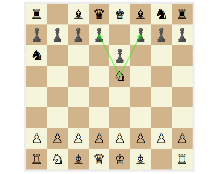
plot of chunk blowup

I looked around for some resources on Atomic chess, but have never had luck with traditional chess studies. Instead I decided to learn about Atomic statistically.

As it happens, Lichess (which is truly a great site) publishes their game data which includes over 9 million Atomic games played. I wrote some code that will download and parse this data, turning it into a CSV file. You can download v1 of this file, but Lichess is the ultimate copyright holder.

First steps

The games in the dataset end in one of three conditions: Normal (checkmate or what passes for it in Atomic), Time forfeit, and Abandoned (game terminated before it began). The last category is very rare, and I omit these from my processing. The majority of games end in the Normal way, as tabulated here:

termination n
Normal 8426052
Time forfeit 1257295

The game data includes Elo scores for players, as computed prior to the game. As a first check, I wanted to see if Elo is properly calibrated. To do this, I compute the empirical win rate of White over Black, grouped by bins of the difference in their Elo …

read more

Nonparametric Market Timing

Sat 04 January 2020 by Steven

Market timing a single instrument with a single feature

read more

Discrete State Market Timing

Sun 30 June 2019 by Steven

Market timing with a discrete feature

read more

Conditional Portfolios with Feature Flattening

Wed 19 June 2019 by Steven E. Pav

Conditional Portfolios

When I first started working at a quant fund I tried to read about portfolio theory. (Beyond, you know, "Hedge Funds for Dummies.") I learned about various objectives and portfolio constraints, including the Markowitz portfolio, which felt very natural. Markowitz solves the mean-variance optimization problem, as well as the Sharpe maximization problem, namely

$$ \operatorname{argmax}_w \frac{w^{\top}\mu}{\sqrt{w^{\top} \Sigma w}}. $$

This is solved, up to scaling, by the Markowitz portfolio \(\Sigma^{-1}\mu\).

When I first read about the theory behind Markowitz, I did not read anything about where \(\mu\) and \(\Sigma\) come from. I assumed the authors I was reading were talking about the vanilla sample estimates of the mean and covariance, though the theory does not require this.

There are some problems with the Markowitz portfolio. For us, as a small quant fund, the most pressing issue was that holding the Markowitz portfolio based on the historical mean and covariance was not a good look. You don't get paid "2 and twenty" for computing some long term averages.

Rather than holding an unconditional portfolio, we sought to construct a conditional one, conditional on some "features". (I now believe this topic falls under the rubric of "Tactical Asset Allocation".) We stumbled on two simple methods for adapting Markowitz theory to accept conditioning information: Conditional Markowitz, and "Flattening".

Conditional Markowitz

Suppose you observe some \(l\) vector of features, \(f_i\) prior to the time you have to allocate into \(p\) assets to enjoy returns \(x_i\). Assume that the returns are linear in the features, but the covariance is a long term average. That is

$$ E\left[x_i \left|f_i\right.\right] = B f_i,\quad\mbox{Var}\left(x_i \left|f_i\right.\right) = \Sigma. $$

Note that Markowitz theory never really said how to estimate mean …

read more