In a previous blog post, I looked at "market timing" for discrete states. There are a number of ways that result can be generalized. Here we consider a non-parametric view. Suppose you observe some scalar feature \(f_t\) prior to the time required to invest and capture scalar returns \(x_{t+1}\). Let \(\mu\left(f\right)\) and \(\alpha_2\left(f\right)\) be the first and second moments of returns conditional on the feature:
Suppose that \(f_t\) is random with density \(g\left(f\right)\).
Suppose that in response to observing \(f_t\) you allocate \(w\left(f_t\right)\) proportion of your wealth long in the asset. The first and second moments of the returns of this strategy are
Now we seek the strategy \(w\left(x\right)\) that maximizes the signal-noise ratio, which is the ratio of the expected return to the standard devation of returns. We can transform this metric to the ratio of expected return to the square root of the second moment, by way of the monotonic 'tas' function (the tangent of the arcsine of the return to square root second moment is the signal-noise ratio). Now note that to maximize this ratio we can, without loss of generality, prespecify the denominator to equal some value. This works because the ratio is homogeneous of order zero, and we can rescale \(w\left(x\right)\) by some arbitrary positive constant and get the same objective. This yields the problem
This, it turns out, is a trivial problem in the calculus of variations. Trivial in the sense that the integrals do not involve the derivative \(w'\left(x\right)\) and so the solution has a simple form which looks just like the finite dimensional Lagrange multiplier solution. After some simplification, the optimal solution is found to be
Note this is fully consistent with what we saw for the case where \(f_t\) took one of a finite set of discrete states in our earlier blog post. However, this doesn't quite look like Markowitz, because the denominator has the second moment function, and not the variance function. We will see this actually matters.
Exponential Heteroskedasticity
As an example, consider the case where \(f_t\) takes an exponential distribution with parameter \(\lambda=1\). Moreover, assume the mean is constant, but the variance is proportional to the feature:
The optimal allocation is
where \(\zeta=\mu/\sigma\). We note that because \(E\left[f_t\right]=1\) and the expected return is constant with respect to \(f_t\), the signal-noise ratio of the buy-and-hold strategy is simply \(\zeta\). The SNR of the optimal timing strategy can be quite a bit higher.
To compute that SNR, first let
(This integral is called the "exponential integral".) Then the SNR of the timing strategy is
Here we confirm this empirically. We spawn a bunch of \(f_t\) and \(x_{t+1}\) under the model, then compute the returns of the buy-and-hold strategy, the optimal strategy, and the Markowitz equivalent which holds proportional to mean divided by variance:
mu <- 0.1
sg <- 1
zetasq <- (mu/sg)^2
set.seed(1234)
feat <- rexp(1e6,rate=1)
rets <- rnorm(length(feat),mean=rep(mu,length(feat)),sd=sg*sqrt(feat))

# optimal allocation;
ww <- 1 / (feat+zetasq)
# markowitz allocation;
mw <- 1 / feat

library(SharpeR)
buyhold <- (as.sr(rets)$sr)
optimal <- (as.sr(rets*ww)$sr)
markwtz <- (as.sr(rets*mw)$sr)

library(expint)
qfunc <- function(zetsq) {
    require(expint,quietly=TRUE)
    zetsq * exp(zetsq) * expint(zetsq)
}
psnrfunc <- function(zetsq) {
    qqq <- qfunc(zetsq)
    sqrt(qqq / (1-qqq))
}
theoretical <- psnrfunc(zetasq)
The empirical SNR of the buy-and-hold strategy is 0.1, which is very close to the theoretical value of 0.1. We compute the SNR of the optimal strategy to be 0.207, which is very close to the theoretical value we compute as 0.206 using the exponential integral above. The signal-noise ratio of the Markowitz strategy, however, is a measly 0.0152.
We note that for this setup, it is simple to find the optimal \(k\) degree polynomial \(w\left(f_t\right)\), and confirm they have lower SNR than what we observe here. We leave that as an exercise in our book.
Timing the Market
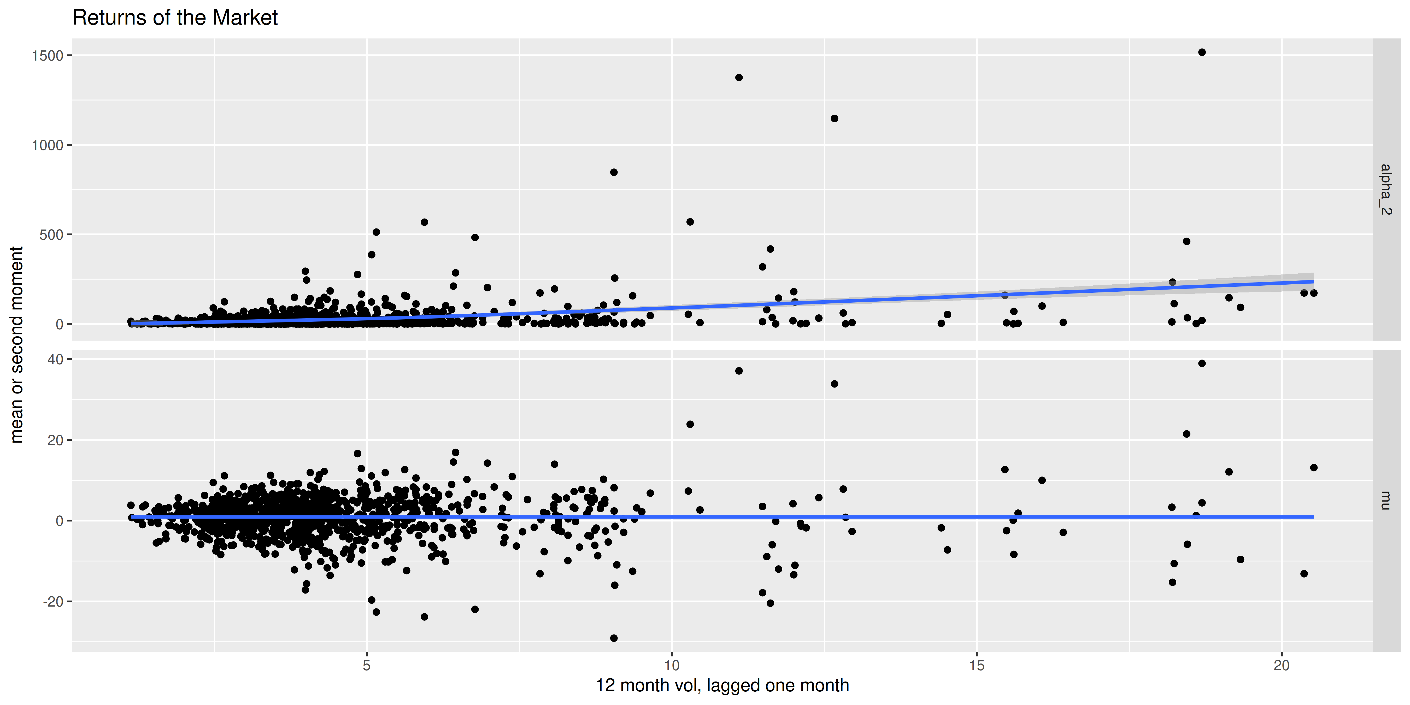
Here we use this technique on returns of the Market, as defined in the Fama-French factors. We take the 12 month rolling volatility of the Market returns, delayed by a month, as our feature. First we plot the market returns and squared market returns as a function of our feature. We see essentially a flat \(\mu\) but an increasing \(\alpha_2\).
suppressMessages({
  library(fromo)
  library(dplyr)
  library(tidyr)
  library(magrittr)
  library(ggplot2)
})

if (!require(aqfb.data) && require(devtools)) {
    devtools::install_github('shabbychef/aqfb_data')
}
library(aqfb.data)
data(mff4)

df <- data.frame(mkt=mff4$Mkt) %>%
  mutate(vol12=as.numeric(fromo::running_sd(Mkt,12,min_df=12L))) %>%
  mutate(feature=dplyr::lag(vol12,2)) %>%
  dplyr::filter(!is.na(feature))

# check on the first moments
ph <- df %>%
    rename(mu=Mkt) %>%
    mutate(alpha_2=mu^2) %>%
    tidyr::gather(key=series,value=value,mu,alpha_2) %>%
    ggplot(aes(feature,value)) +
    geom_point() +
    stat_smooth() +
    facet_grid(series~.,scales='free') +
    labs(x='12 month vol, lagged one month',
             y='mean or second moment',
             title='Returns of the Market')
print(ph)

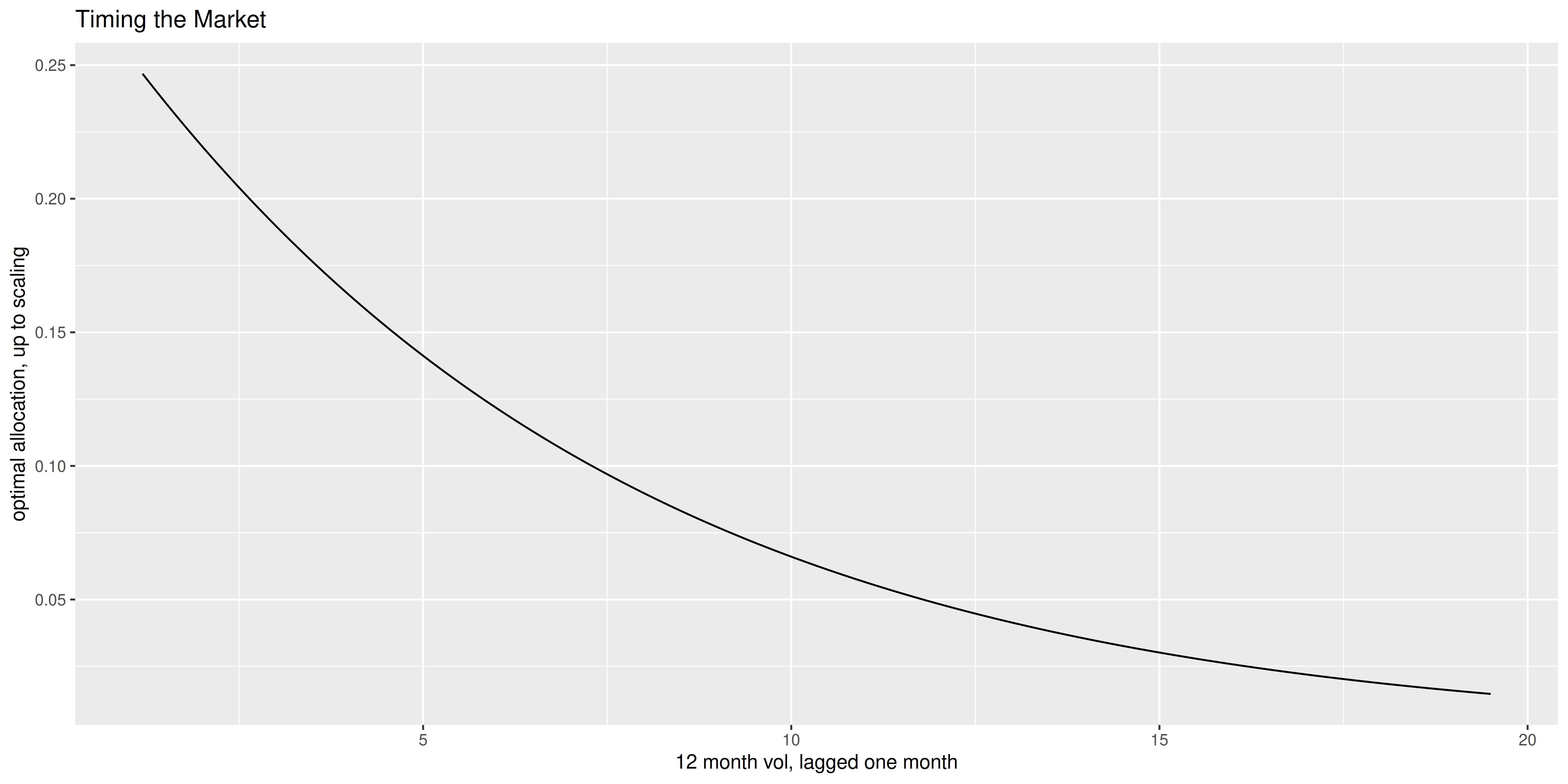
We now perform a GAM fit on the first and second moments of the Market returns. I have to use a trick to force the second moment estimate to be positive. I plot the optimal allocation versus the feature below. Note that it vaguely resembles the optimal allocation from the exponential heteroskedasticity toy example above. One could also estimate the SNR one would achieve in this case, but that ignores the effects of any estimation error. Moreover, the multi-period SNR that we compute here might be considered a very long term average, something that might not be terribly noticeable on a short time scale.
# do two fits
suppressMessages({
    library(mgcv)
})
spn <- 0.9
mufunc <- mgcv::gam(Mkt ~ feature,data=df,family=gaussian())
a2func <- mgcv::gam(I(log(pmax(1e-6,Mkt^2))) ~ feature,data=df,family=gaussian())
alloc <- tibble(feature=seq(min(df$feature)*1.05,max(df$feature)*0.95,length.out=501)) %>%
    mutate(wts=predict(mufunc,.) / exp(predict(a2func,.)))

# if you wanted to estimate the SNR of this allocation:
df2 <- df %>%
    mutate(wts=predict(mufunc,.) / exp(predict(a2func,.))) %>%
    mutate(ret=Mkt * wts)
zetfoo <- as.sr(df2$ret,ope=12)

ph <- alloc %>%
    ggplot(aes(feature,wts)) +
    geom_line() +
    labs(x='12 month vol, lagged one month',
             y='optimal allocation, up to scaling',
             title='Timing the Market')
print(ph)

Checking on leverage
One odd way to use this nonparametric market timing trick in quantitative trading (though do not take this as investing advice!) is as a kind of check on the leverage of a strategy that levers itself. That is, suppose you have some kind of quantitative strategy that does not always use all the capital allocated to it. Let \(f_t\) be the proportion of wealth that the strategy 'decides' to allocate. Of course this is observable prior to the investment decision. Then estimate, nonparametrically, the first and second moment of the returns of the strategy on full leverage from historical returns. Then compute the optimal leverage as a function of the allocated leverage, and plot one against the other: they should fall on a straight line! If they do not fall on a straight line, the strategy is not making optimal decisions regarding leverage (modulo estimation error).